For those in the scientific world, grappling with complex numerical problems is a common experience. Whether you're an engineer, physicist, or data analyst, having the right tools at your disposal is crucial. This is where GNU Octave comes in.
What is GNU Octave?
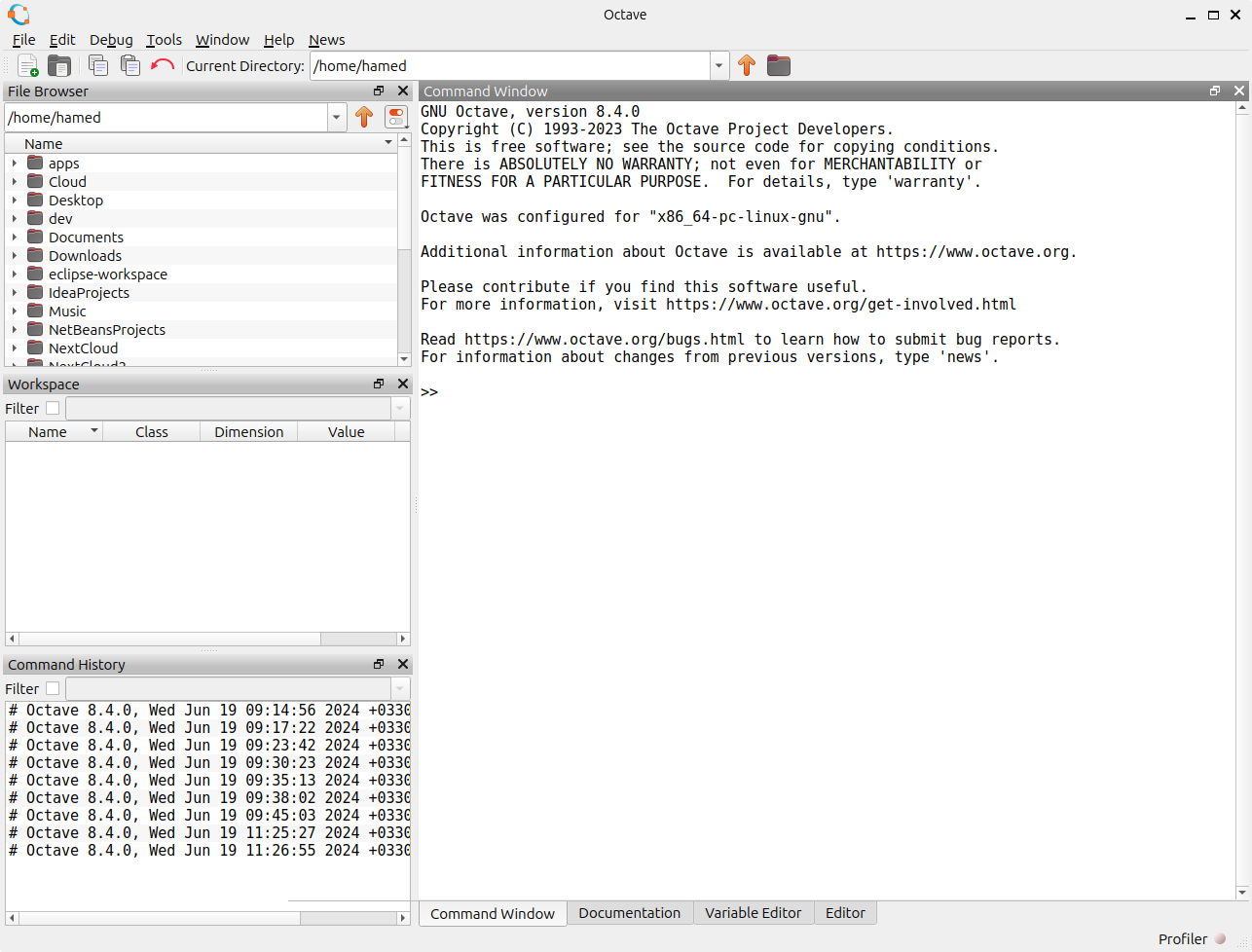
GNU Octave is a free, open-source programming language specifically designed for scientific computing. It empowers you to tackle numerical computations, solve linear and non-linear problems, and visualize data with ease. One of its biggest strengths is its compatibility with MATLAB, another popular scientific software program. This means that if you're already familiar with MATLAB, the transition to Octave will be smooth.

Why Choose GNU Octave?
There are several compelling reasons to consider GNU Octave for your scientific computing needs:
- Free and Open-Source: Unlike some commercial software, Octave won't break the bank. Since it's open-source, you have the freedom to modify and distribute the code as needed.
- Powerful Functionality: Octave boasts a rich set of features for numerical computations, linear algebra, data analysis, and visualization.
- Extensible with Packages: The functionality of Octave can be further enhanced by installing packages from the Octave Forge repository. These packages cater to specific scientific domains, giving you even more problem-solving power.
- Runs on Multiple Platforms: GNU Octave is available for Windows, macOS, Linux, and BSD operating systems, providing great flexibility.
Getting Started with GNU Octave
If you're tertarik ( tertarik is Indonesian for interested) in giving GNU Octave a try, the good news is it's easy to get started. Head over to the official GNU Octave website [GNU Octave] to download the software for your specific operating system. The website also offers comprehensive documentation and tutorials to help you navigate the world of Octave programming.
Beyond the Basics
Once you're comfortable with the fundamentals, the Octave online community provides a wealth of resources for further exploration. You'll find forums, discussions, and even online platforms like Octave Online [Octave Online] that allow you to run Octave directly in your web browser.
Embrace the Power of Free Scientific Computing
GNU Octave is a fantastic option for anyone looking for a powerful, free, and user-friendly scientific computing environment. So why not dive in and see what it can do for your next scientific project?
Octave's Capabilities at Your Fingertips
GNU Octave packs a powerful punch when it comes to scientific computing. Here's a quick rundown of its capabilities:
- Numerical computations: Octave excels at performing complex calculations, from basic arithmetic to solving advanced mathematical equations.
- Linear algebra: It provides a comprehensive set of tools for manipulating matrices, solving linear systems, and performing eigenvalue analysis.
- Data analysis: Octave equips you with functions for data import, filtering, transformation, and statistical analysis.
- Visualization: Create informative graphs and plots to visualize your data, including 2D and 3D plots.
- Extensibility: Expand Octave's potential with a vast library of packages from the Octave Forge, tackling specialized problems in various scientific fields.
Exploring Octave with Basic Examples
GNU Octave offers a user-friendly interface for various scientific tasks. Let's jump into some simple examples to get a taste of its capabilities:
Basic Arithmetic:
a = 5;
b = 2;

# Addition
sum = a + b;

# Subtraction
difference = a - b;

# Multiplication
product = a * b;

# Division
quotient = a / b;

disp("Sum: "), disp(sum)
disp("Difference: "), disp(difference)
disp("Product: "), disp(product)
disp("Quotient: "), disp(quotient)
This code defines variables, performs basic arithmetic operations, and displays the results using the disp function.
Creating and Manipulating Matrices:
# Define a matrix
A = [1 2 3; 4 5 6];

# Access elements
element = A(2, 1);  # element at row 2, column 1

# Modify elements
A(1, 2) = 10;

# Display the matrix
disp("Matrix A: ")
disp(A)
This example demonstrates creating a matrix, accessing individual elements, modifying them, and displaying the entire matrix.
Using Built-in Mathematical Functions:
x = 2;

# Calculate sine
sine_value = sin(x);

# Calculate square root
square_root = sqrt(x);

disp("Sine of 2: "), disp(sine_value)
disp("Square root of 2: "), disp(square_root)
This code showcases using built-in functions like sin and sqrt for trigonometric and mathematical operations.
Simple Plotting:
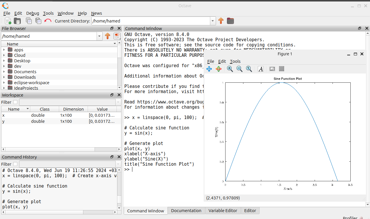
x = linspace(0, pi, 100);  # Create x-axis values

# Calculate sine function
y = sin(x);

# Generate plot
plot(x, y)
xlabel("X-axis")
ylabel("Sine(X)")
title("Sine Function Plot")
This example utilizes the linspace function to create an array of x-values, calculates the sine function for those values, and uses the plot function to generate a visual representation.

These are just a few basic examples to get you started with GNU Octave. As you explore further, you'll discover its vast potential for tackling more complex scientific problems.
Delving Deeper: Complex Examples in Octave
While the previous examples showcased Octave's basics, here's a glimpse into its capabilities for more intricate tasks:
Solving Linear Systems:
# Define a coefficient matrix and constant vector
A = [2 1; 1 3];
b = [5; 8];

# Solve for the solution vector x
x = A \ b;

disp("Solution vector x: ")
disp(x)
This example defines a system of linear equations represented by a matrix equation Ax = b. The backslash operator (\) is used to solve for the unknown vector x.
Symbolic Math:
# Define symbolic variables
syms x y

# Symbolic expression
eqn = x^2 + y^2 - 4;

# Solve for symbolic roots
sol = solve(eqn, x);

disp("Symbolic roots of x: ")
disp(sol)
This example ventures into symbolic math. We define symbolic variables x and y, create a symbolic expression, and utilize the solve function to find the symbolic roots for x.
Data Analysis with Statistics:
# Sample data
data = [2, 5, 7, 1, 8, 3, 9];

# Mean, standard deviation, and median
mean_value = mean(data);
std_dev = std(data);
median_value = median(data);

disp("Mean: "), disp(mean_value)
disp("Standard Deviation: "), disp(std_dev)
disp("Median: "), disp(median_value)
Here, we demonstrate data analysis functionalities. Sample data is created, and functions like mean, std, and median are used to calculate statistical properties.
Visualization with Customization:
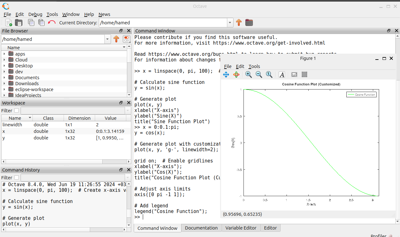
x = 0:0.1:pi;
y = cos(x);

# Generate plot with customization
plot(x, y, 'g-', linewidth=2);  # Green line, thicker

grid on;  # Enable gridlines
xlabel("X-axis");
ylabel("Cos(X)");
title("Cosine Function Plot (Customized)");

# Adjust axis limits
axis([0 pi -1 1]);

# Add legend
legend("Cosine Function");
This example builds upon the basic plotting example, incorporating customizations. Line color, thickness, gridlines, axis limits, and legends are included to enhance the visualization.

Utilizing Octave Forge Packages:
Let's say you're working with audio signals. Octave doesn't have built-in functions for everything. Here's where Octave Forge comes in.
# Install the signal package from Octave Forge
pkg install -forge signal

# Load a sample audio file
[y, Fs] = wavread("sample.wav");

# Plot the audio signal
plot(y(1:1000))
xlabel("Sample Number")
ylabel("Amplitude")
title("Sample Audio Signal")

# Analyze the signal using functions from the signal package
# ... (Further code using signal processing functions)
This example highlights the power of Octave Forge. We install the signal package, enabling functionalities for audio processing. We can then load and plot an audio signal, and use functions from the package for further analysis.
These are just a few examples showcasing Octave's potential for complex scientific tasks. With its extensive functionalities and available packages, Octave empowers you to tackle a wide range of computational challenges.